Deep TT Density demo

The torchtt.nn.TTDensityLayer represents a probability density as a normalized squared functional Tensor Train — a “Born-machine” density.

Given univariate basis functions \(\{\phi^{(k)}_i\}_{i=1}^{N_k}\) for every dimension \(k = 1, \dots, d\) (here Gaussians), we build a scalar model function

\[f(x_1, \dots, x_d) = \sum_{i_1=1}^{N_1} \cdots \sum_{i_d=1}^{N_d} G_{i_1 \dots i_d}\, \phi^{(1)}_{i_1}(x_1) \cdots \phi^{(d)}_{i_d}(x_d),\]

whose coefficient tensor \(G\) is stored in the Tensor-Train format with cores \(G^{(k)} \in \mathbb{R}^{R_k \times N_k \times R_{k+1}}\) and \(R_1 = R_{d+1} = 1\). The density is the normalized square

\[p_\text{ref}(x) = \frac{f(x)^2}{\int f(y)^2\, dy}.\]

Squaring guarantees non-negativity, and the normalizer \(Z = \int f^2\) is available in closed form from the cores and the basis integration weights \(w^{(k)}_i = \int \phi^{(k)}_i\), so \(p_\text{ref}\) integrates to \(1\) by construction.

Optionally a diffeomorphism \(T\) (a smooth, invertible change of variables) is applied, yielding the push-forward density through the change-of-variables formula

\[p(x) = p_\text{ref}\big(T(x)\big)\, \big|\det J_T(x)\big|.\]

The transform lets a low-rank reference density represent correlated or curved distributions. Because the cores are meant to be produced by an upstream neural network (hence deep TT), the layer is an ordinary torch.nn.Module: it takes a flat parameter vector — the flattened TT cores followed by the transform parameters — together with the evaluation points \(x\), and returns \(p(x)\). A network can thus emit a different density for every element of a batch.

%matplotlib inline
import torch
import matplotlib.pyplot as plt

import torchtt
import torchtt.functional
from torchtt.nn import (
    TTDensityLayer,
    AffineTransform,
    Rank1Shear,
    SinhArcsinhWarp,
    TriangularPolyShear,
    ComposedTransform,
)

The reference density: basis and layer

We work in \(d = 2\). Each dimension is given a Gaussian basis centred on a uniform grid of \(N_k\) points on \([0, 1]\); delta_overlap=1 sets every Gaussian’s width to the spacing of its immediate neighbour, so adjacent bumps overlap smoothly. The TT ranks R = [1, 5, 1] allow a bond rank of \(5\) between the two modes, which controls how much correlation between \(x_1\) and \(x_2\) the density can capture.

The flattened TT cores contain \(\sum_k R_k N_k R_{k+1}\) numbers; we draw them once as theta_core and reuse this single reference density throughout, appending a different transform’s parameters after it in each section below.

torch.manual_seed(0)

dim = 2
N = [10, 11]          # number of basis functions per dimension
R = [1, 5, 1]         # TT ranks (bond rank 5 between the two modes)

basis = [
    torchtt.functional.GaussianBasis(torch.linspace(0, 1, N[0]), delta_overlap=1),
    torchtt.functional.GaussianBasis(torch.linspace(0, 1, N[1]), delta_overlap=1),
]

# The flattened TT cores have this many entries; every layer below appends its
# own transform parameters after them.
n_core = sum(n * r0 * r1 for n, r0, r1 in zip(N, R, R[1:]))
theta_core = torch.rand(n_core)   # one shared reference density, reused everywhere

print(f"TT-core parameters: {n_core}")

TT-core parameters: 105

Checking the normalization

The flat input vector is laid out as \([\,\text{TT cores}\ |\ \text{transform params}\,]\). We are not training here, so we simply draw one random parameter vector (the shared cores plus a random affine transform \(z = R(\theta)\,\mathrm{diag}(e^{a})\,x + b\)), broadcast it across a batch of \(M = 2^{18}\) points, and confirm the density is normalized with a Monte-Carlo estimate

\[\int_\Omega p(x)\, dx \;\approx\; \frac{|\Omega|}{M} \sum_{m=1}^{M} p\big(x^{(m)}\big), \qquad x^{(m)} \sim \mathrm{Unif}(\Omega),\]

on a square \(\Omega\) of area \(|\Omega| = 3^2\) centred on the affine offset \(b\) so it sits over the density’s mass. The estimate should come out close to \(1\).

transform = AffineTransform(dim)
layer = TTDensityLayer(N, R, basis, transform=transform)

n_samples = 2**18
theta_affine = torch.rand(transform.input_requirement())
params = torch.cat([theta_core, theta_affine])
offset = theta_affine[-dim:]                       # the affine translation b

tts = params.unsqueeze(0).expand(n_samples, -1)
box = 3.0
xs = torch.rand(n_samples, dim) * box - box / 2 + offset   # box centred on the mass
pdf_val = layer(tts, xs)

integral = pdf_val.sum() / n_samples * box**dim
print("pdf batch shape:", tuple(pdf_val.shape))
print(f"Monte-Carlo integral (expected ~1): {integral:.4f}")

pdf batch shape: (262144,)
Monte-Carlo integral (expected ~1): 1.0053

Transformation and density

From here on we tour the diffeomorphisms available in torchtt.nn. Each one plugs into a TTDensityLayer the same way, so we keep the same reference cores theta_core and only change the transform tail.

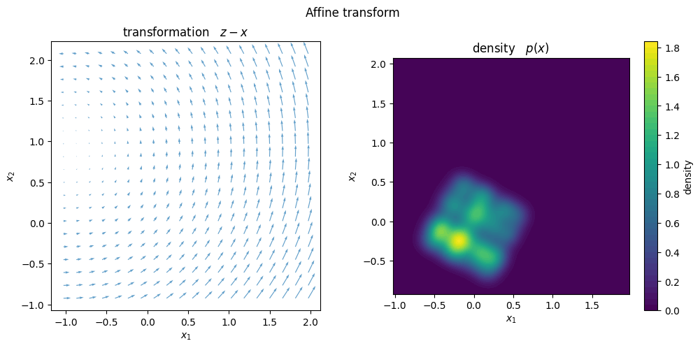
For every transform we draw two panels over a common window: on the left the displacement field \(z - x = T(x) - x\) (how the map moves points), and on the right the resulting density \(p(x) = p_\text{ref}(T(x))\,|\det J_T(x)|\). We start with the affine map used above.

# Reuse the affine transform, layer and parameters from the check above.
print(f"TT-core parameters:   {n_core}")
print(f"transform parameters: {transform.input_requirement()}")

x0, x1 = offset[0].item() - 1.5, offset[0].item() + 1.5
y0, y1 = offset[1].item() - 1.5, offset[1].item() + 1.5

# left panel: the transformation's displacement field  z - x  (20 x 20 grid)
qx, qy = torch.linspace(x0, x1, 20), torch.linspace(y0, y1, 20)
Xq, Yq = torch.meshgrid(qx, qy, indexing="ij")
grid_q = torch.stack((Xq.flatten(), Yq.flatten()), dim=1)
z, _ = transform(grid_q, theta_affine.expand(grid_q.shape[0], -1))
U = (z[:, 0] - grid_q[:, 0]).reshape(20, 20)
V = (z[:, 1] - grid_q[:, 1]).reshape(20, 20)

# right panel: the density  p(x)  (200 x 200 grid)
gx, gy = torch.linspace(x0, x1, 200), torch.linspace(y0, y1, 200)
Xg, Yg = torch.meshgrid(gx, gy, indexing="ij")
grid_g = torch.stack((Xg.flatten(), Yg.flatten()), dim=1)
full_params = torch.cat([theta_core, theta_affine])
with torch.no_grad():
    pdf = layer(full_params.unsqueeze(0).expand(grid_g.shape[0], -1), grid_g).reshape(200, 200)

fig, (ax_t, ax_p) = plt.subplots(1, 2, figsize=(12, 5))
ax_t.quiver(Xq.numpy(), Yq.numpy(), U.numpy(), V.numpy(), color="tab:blue", alpha=0.7)
ax_t.set_title("transformation   $z - x$")
cf = ax_p.contourf(Xg.numpy(), Yg.numpy(), pdf.numpy(), levels=50)
fig.colorbar(cf, ax=ax_p, label="density")
ax_p.set_title("density   $p(x)$")
for ax in (ax_t, ax_p):
    ax.set_xlabel("$x_1$")
    ax.set_ylabel("$x_2$")
    ax.set_aspect("equal")
fig.suptitle("Affine transform")
plt.show()

TT-core parameters:   105
transform parameters: 5

Rank-1 shear

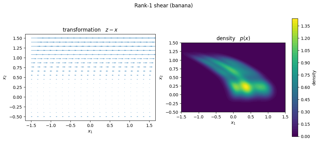
At low rank the reference density is restricted to fairly generic shapes (roughly a rotated, scaled blob). A nonlinear diffeomorphism can bend it into curved distributions such as the classic “banana”.

Rank1Shear is a volume-preserving rank-1 shear

\[z = x + u\, g(v^\top x + c), \qquad g(t) = \sum_{p=1}^{D} \alpha_p\, t^p,\]

where \(u\) is internally projected orthogonally to \(v\) so that \(v^\top u = 0\) and hence \(\det J = 1\). With \(u = [1, 0]\), \(v = [0, 1]\), \(c = 0\) and \(g(t) = t^2\) it becomes \((x_1, x_2) \mapsto (x_1 + x_2^2,\ x_2)\) — a parabolic shear along the first axis, with parameter vector \([u_x, u_y, v_x, v_y, c, \alpha_1, \alpha_2]\).

shear = Rank1Shear(dim, degree=2)
layer_shear = TTDensityLayer(N, R, basis, transform=shear)

# [u_x, u_y, v_x, v_y, c, alpha_1, alpha_2]:  u=[1,0], v=[0,1], g(t)=t**2
shear_params = torch.tensor([1.0, 0.0, 0.0, 1.0, 0.0, 0.0, 1.0])

print(f"TT-core parameters:   {n_core}")
print(f"transform parameters: {shear.input_requirement()}")

x0, x1, y0, y1 = -1.5, 1.5, -0.5, 1.5

# left panel: the transformation's displacement field  z - x  (20 x 20 grid)
qx, qy = torch.linspace(x0, x1, 20), torch.linspace(y0, y1, 20)
Xq, Yq = torch.meshgrid(qx, qy, indexing="ij")
grid_q = torch.stack((Xq.flatten(), Yq.flatten()), dim=1)
z, _ = shear(grid_q, shear_params.expand(grid_q.shape[0], -1))
U = (z[:, 0] - grid_q[:, 0]).reshape(20, 20)
V = (z[:, 1] - grid_q[:, 1]).reshape(20, 20)

# right panel: the density  p(x)  (200 x 200 grid)
gx, gy = torch.linspace(x0, x1, 200), torch.linspace(y0, y1, 200)
Xg, Yg = torch.meshgrid(gx, gy, indexing="ij")
grid_g = torch.stack((Xg.flatten(), Yg.flatten()), dim=1)
full_params = torch.cat([theta_core, shear_params])
with torch.no_grad():
    pdf = layer_shear(full_params.unsqueeze(0).expand(grid_g.shape[0], -1), grid_g).reshape(200, 200)

fig, (ax_t, ax_p) = plt.subplots(1, 2, figsize=(12, 5))
ax_t.quiver(Xq.numpy(), Yq.numpy(), U.numpy(), V.numpy(), color="tab:blue", alpha=0.7)
ax_t.set_title("transformation   $z - x$")
cf = ax_p.contourf(Xg.numpy(), Yg.numpy(), pdf.numpy(), levels=50)
fig.colorbar(cf, ax=ax_p, label="density")
ax_p.set_title("density   $p(x)$")
for ax in (ax_t, ax_p):
    ax.set_xlabel("$x_1$")
    ax.set_ylabel("$x_2$")
    ax.set_aspect("equal")
fig.suptitle("Rank-1 shear (banana)")
plt.show()

TT-core parameters:   105
transform parameters: 7

Sinh-arcsinh warp

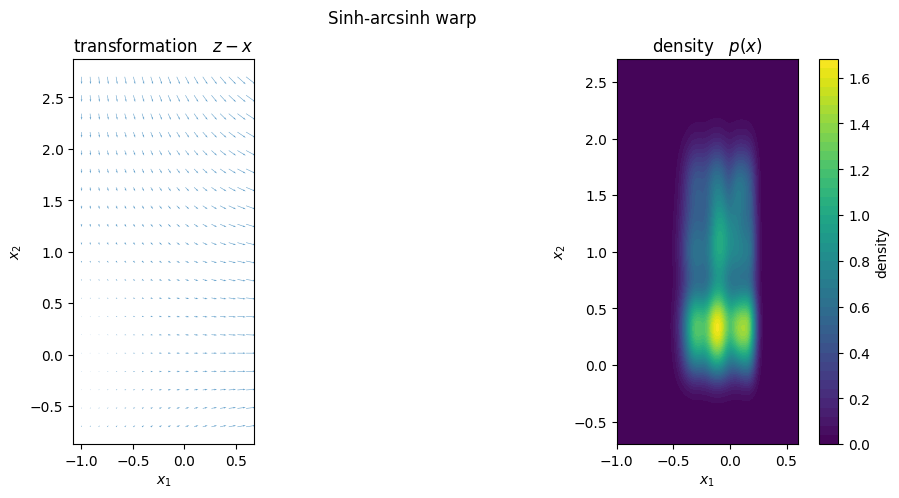
SinhArcsinhWarp acts on each coordinate independently,

\[z_i = \sinh\!\big(e^{s_i}\,\operatorname{asinh}(x_i) + b_i\big),\]

with per-axis parameters \([s_1, s_2, b_1, b_2]\). The offset \(b_i\) controls the skewness and the log-scale \(s_i\) the tail weight along axis \(i\). Unlike the shears it has a non-trivial Jacobian, \(\det J = \prod_i e^{s_i}\cosh(\cdot)/\sqrt{1 + x_i^2}\).

warp = SinhArcsinhWarp(dim)
layer_warp = TTDensityLayer(N, R, basis, transform=warp)

# [s_1, s_2, b_1, b_2]:  per-axis log-scale (tails) and offset (skew)
warp_params = torch.tensor([0.5, -0.4, 0.6, 0.0])

print(f"TT-core parameters:   {n_core}")
print(f"transform parameters: {warp.input_requirement()}")

x0, x1, y0, y1 = -1.0, 0.6, -0.7, 2.7

# left panel: the transformation's displacement field  z - x  (20 x 20 grid)
qx, qy = torch.linspace(x0, x1, 20), torch.linspace(y0, y1, 20)
Xq, Yq = torch.meshgrid(qx, qy, indexing="ij")
grid_q = torch.stack((Xq.flatten(), Yq.flatten()), dim=1)
z, _ = warp(grid_q, warp_params.expand(grid_q.shape[0], -1))
U = (z[:, 0] - grid_q[:, 0]).reshape(20, 20)
V = (z[:, 1] - grid_q[:, 1]).reshape(20, 20)

# right panel: the density  p(x)  (200 x 200 grid)
gx, gy = torch.linspace(x0, x1, 200), torch.linspace(y0, y1, 200)
Xg, Yg = torch.meshgrid(gx, gy, indexing="ij")
grid_g = torch.stack((Xg.flatten(), Yg.flatten()), dim=1)
full_params = torch.cat([theta_core, warp_params])
with torch.no_grad():
    pdf = layer_warp(full_params.unsqueeze(0).expand(grid_g.shape[0], -1), grid_g).reshape(200, 200)

fig, (ax_t, ax_p) = plt.subplots(1, 2, figsize=(12, 5))
ax_t.quiver(Xq.numpy(), Yq.numpy(), U.numpy(), V.numpy(), color="tab:blue", alpha=0.7)
ax_t.set_title("transformation   $z - x$")
cf = ax_p.contourf(Xg.numpy(), Yg.numpy(), pdf.numpy(), levels=50)
fig.colorbar(cf, ax=ax_p, label="density")
ax_p.set_title("density   $p(x)$")
for ax in (ax_t, ax_p):
    ax.set_xlabel("$x_1$")
    ax.set_ylabel("$x_2$")
    ax.set_aspect("equal")
fig.suptitle("Sinh-arcsinh warp")
plt.show()

TT-core parameters:   105
transform parameters: 4

Triangular polynomial shear

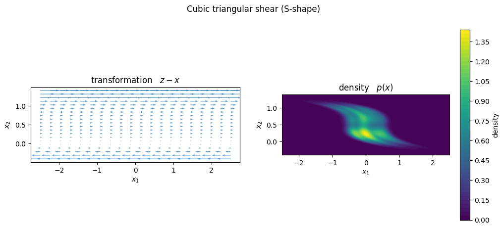
TriangularPolyShear is a Knothe-Rosenblatt map: each coordinate is shifted by a polynomial of the later coordinates,

\[z_i = x_i + \sum_{j>i} q_{ij}(x_j), \qquad q_{ij}(t) = \sum_{p=1}^{D} \beta_{ij,p}\, t^p,\]

which is triangular and hence volume-preserving (\(\det J = 1\)). In 2-D a single polynomial \(q(x_2)\) shifts \(x_1\); where the banana used \(q(t) = t^2\), a cubic \(q\) can bend the density into an S-shape.

poly_shear = TriangularPolyShear(dim, degree=3)
layer_poly = TTDensityLayer(N, R, basis, transform=poly_shear)

# [beta_1, beta_2, beta_3]:  q(t) = beta_1 t + beta_2 t**2 + beta_3 t**3
poly_params = torch.tensor([3.0, -6.0, 4.0])

print(f"TT-core parameters:   {n_core}")
print(f"transform parameters: {poly_shear.input_requirement()}")

x0, x1, y0, y1 = -2.5, 2.5, -0.4, 1.4

# left panel: the transformation's displacement field  z - x  (20 x 20 grid)
qx, qy = torch.linspace(x0, x1, 20), torch.linspace(y0, y1, 20)
Xq, Yq = torch.meshgrid(qx, qy, indexing="ij")
grid_q = torch.stack((Xq.flatten(), Yq.flatten()), dim=1)
z, _ = poly_shear(grid_q, poly_params.expand(grid_q.shape[0], -1))
U = (z[:, 0] - grid_q[:, 0]).reshape(20, 20)
V = (z[:, 1] - grid_q[:, 1]).reshape(20, 20)

# right panel: the density  p(x)  (200 x 200 grid)
gx, gy = torch.linspace(x0, x1, 200), torch.linspace(y0, y1, 200)
Xg, Yg = torch.meshgrid(gx, gy, indexing="ij")
grid_g = torch.stack((Xg.flatten(), Yg.flatten()), dim=1)
full_params = torch.cat([theta_core, poly_params])
with torch.no_grad():
    pdf = layer_poly(full_params.unsqueeze(0).expand(grid_g.shape[0], -1), grid_g).reshape(200, 200)

fig, (ax_t, ax_p) = plt.subplots(1, 2, figsize=(12, 5))
ax_t.quiver(Xq.numpy(), Yq.numpy(), U.numpy(), V.numpy(), color="tab:blue", alpha=0.7)
ax_t.set_title("transformation   $z - x$")
cf = ax_p.contourf(Xg.numpy(), Yg.numpy(), pdf.numpy(), levels=50)
fig.colorbar(cf, ax=ax_p, label="density")
ax_p.set_title("density   $p(x)$")
for ax in (ax_t, ax_p):
    ax.set_xlabel("$x_1$")
    ax.set_ylabel("$x_2$")
    ax.set_aspect("equal")
fig.suptitle("Cubic triangular shear (S-shape)")
plt.show()

TT-core parameters:   105
transform parameters: 3

Composing transforms

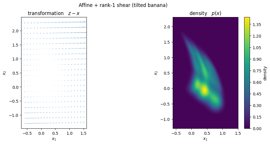
ComposedTransform chains several diffeomorphisms, applying them in order and multiplying their Jacobian determinants; its parameter vector is simply the concatenation of the individual ones. Here an affine rotation is followed by the rank-1 shear, producing a tilted banana.

composed = ComposedTransform([AffineTransform(dim), Rank1Shear(dim, degree=2)])
layer_comp = TTDensityLayer(N, R, basis, transform=composed)

# affine rotation by 0.7 rad, then the banana shear (parameters concatenated)
affine_rot = torch.tensor([0.7, 0.0, 0.0, 0.0, 0.0])
shear_bend = torch.tensor([1.0, 0.0, 0.0, 1.0, 0.0, 0.0, 1.0])
comp_params = torch.cat([affine_rot, shear_bend])

print(f"TT-core parameters:   {n_core}")
print(f"transform parameters: {composed.input_requirement()}")

x0, x1, y0, y1 = -0.6, 1.5, -1.3, 2.3

# left panel: the transformation's displacement field  z - x  (20 x 20 grid)
qx, qy = torch.linspace(x0, x1, 20), torch.linspace(y0, y1, 20)
Xq, Yq = torch.meshgrid(qx, qy, indexing="ij")
grid_q = torch.stack((Xq.flatten(), Yq.flatten()), dim=1)
z, _ = composed(grid_q, comp_params.expand(grid_q.shape[0], -1))
U = (z[:, 0] - grid_q[:, 0]).reshape(20, 20)
V = (z[:, 1] - grid_q[:, 1]).reshape(20, 20)

# right panel: the density  p(x)  (200 x 200 grid)
gx, gy = torch.linspace(x0, x1, 200), torch.linspace(y0, y1, 200)
Xg, Yg = torch.meshgrid(gx, gy, indexing="ij")
grid_g = torch.stack((Xg.flatten(), Yg.flatten()), dim=1)
full_params = torch.cat([theta_core, comp_params])
with torch.no_grad():
    pdf = layer_comp(full_params.unsqueeze(0).expand(grid_g.shape[0], -1), grid_g).reshape(200, 200)

fig, (ax_t, ax_p) = plt.subplots(1, 2, figsize=(12, 5))
ax_t.quiver(Xq.numpy(), Yq.numpy(), U.numpy(), V.numpy(), color="tab:blue", alpha=0.7)
ax_t.set_title("transformation   $z - x$")
cf = ax_p.contourf(Xg.numpy(), Yg.numpy(), pdf.numpy(), levels=50)
fig.colorbar(cf, ax=ax_p, label="density")
ax_p.set_title("density   $p(x)$")
for ax in (ax_t, ax_p):
    ax.set_xlabel("$x_1$")
    ax.set_ylabel("$x_2$")
    ax.set_aspect("equal")
fig.suptitle("Affine + rank-1 shear (tilted banana)")
plt.show()

TT-core parameters:   105
transform parameters: 12